num_data_points <- 5

mean_data <- 3.0
sd_data <- 1.0
new_data <- rnorm(num_data_points, mean = mean_data, sd = sd_data)14 Parameter calibration using Bayesian methods
Including parameter uncertainty in forecasts, as demonstrated in Section 17.2, requires having a probability distribution for the parameters. The previous chapter shows how to estimate parameters using likelihood methods. While likelihood methods are designed to find optimal values, they are not designed to estimate the probability distribution of the parameters. By finding optimal values likelihood methods can reduce process uncertainty because a better calibrated model has a better match to historical data and smaller residual error. This chapter introduces the use of Bayesian methods to estimate parameter distributions.
14.1 Introduction to Bayesian statistics
14.1.1 Starting with likelihood
Here we start where we left off with the likelihood chapter Chapter 13. Imagine the following dataset with five data points drawn from a normal distribution (Figure 14.1).
hist(new_data, main = "")
We can calculate the likelihood for a set of different means using the manual likelihood estimation that we did in Chapter 13.
#DATA MODEL
delta_x <- 0.1
x <- seq(-10,10, delta_x)
negative_log_likelihood <- rep(NA,length(x))

for(i in 1:length(x)){
  negative_log_likelihood[i] <- -sum(dnorm(new_data, mean = x[i], sd = 1, log = TRUE))
}
Figure 14.2 is the likelihood surface for different values of the mean given the observation of x = 2.
plot(x, negative_log_likelihood)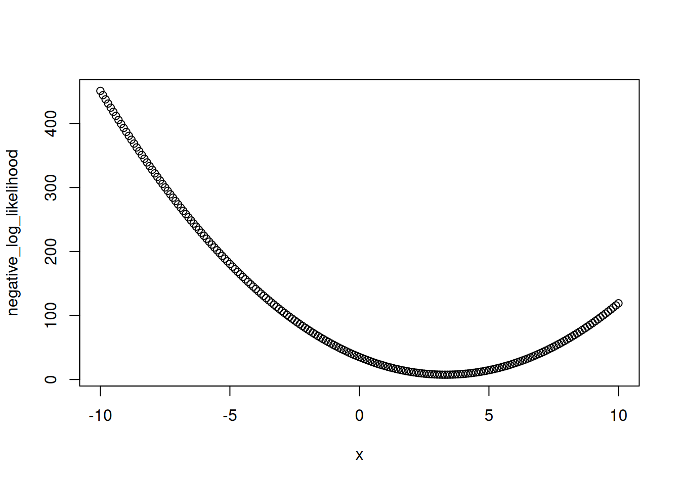
The negative log-likelihood is useful for finding the maximum likelihood values with an optimizing function. However, here we want to convert back to a density (Figure 14.3)
density_likelihood <- exp(-negative_log_likelihood)plot(x, density_likelihood, type = "l")
The y-axis is a tiny number because we multiplied probability densities together. This is OK for our illustrative purposes. To help visualize we can rescale so that the area under the curve is 1. The area is approximated where the density is the height and the width is the distance between points on the x-axis (delta_x) that we evaluated (height x width is the area of a bar under the curve). If we sum the bars together, we get the area under the curve (a value way less than 1). Dividing the likelihood by the area rescales the densities so the area under the curve is 1. Rescaling the likelihood is not a formal part of the analysis - just used here for visualizing.
likelihood_area_under_curve <- sum(density_likelihood * delta_x) #Width * Height

density_likelihood_rescaled <- density_likelihood/likelihood_area_under_curve
The rescaled likelihood looks like this (Figure 14.4)
d <- tibble(x = x,
            likelihood = density_likelihood_rescaled)
ggplot(data = d, aes(x = x, y = likelihood)) +
  geom_line() +
  theme_bw()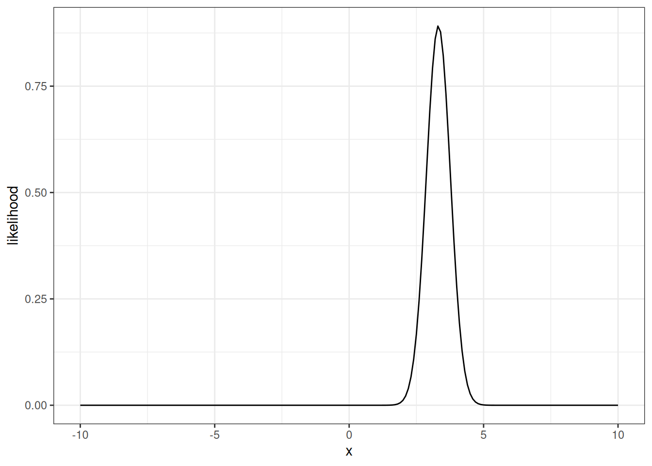
Remember that this curve is the \(P(data \| mean = x)\) - the probability of the data given the model. We want the \(P(mean = x \| data)\) - probability of the model given the data.
Following Bayes rule where the \(P(data | model)\) is the likelihood and \(P(model)\) is our guess for the mean before seeing the data (called the prior)
\[ P(model | data) = \frac{P(data | model) \cdot P(model)}{P(data)} \]
we can multiply the likelihood x the prior.
\[ P(mean | data) \simeq likelihood \cdot prior \] Our prior is the following normal distribution
mean_prior <- 0
sd_prior <- 1.0
With the density for each value of x in Figure 14.5
density_prior <- dnorm(x, mean = mean_prior, sd = sd_prior)d <- tibble(x = x,
density_prior = density_prior)
ggplot(d, aes(x = x, y = density_prior)) +
geom_line() +
theme_bw()
Putting the rescaled likelihood on the same plot as the prior results in Figure 14.6
tibble(x = x,
            prior = density_prior,
            likelihood_rescaled = density_likelihood_rescaled) %>%
  pivot_longer(cols = -x, names_to = "distribution", values_to = "density") %>%
  mutate(distribution = factor(distribution)) %>%
  ggplot(aes(x = x, y = density, color = distribution)) +
  geom_line()  +
  theme_bw()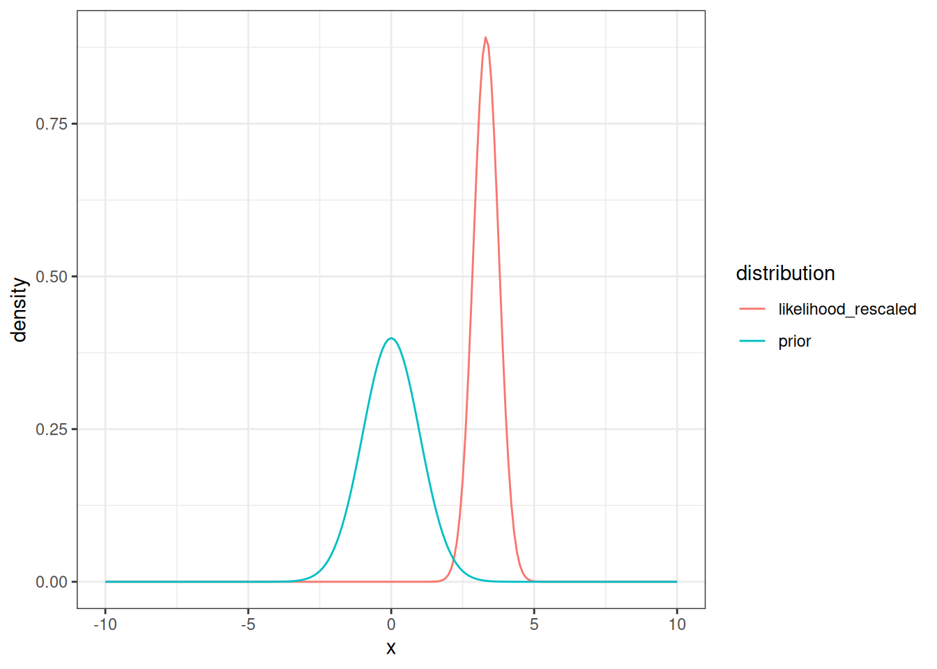
Multiplying the prior x the likelihood (not rescaled) gives Figure 14.7
prior_times_likelihood <- density_prior * density_likelihoodd <- tibble(x = x,
prior_times_likelihood = prior_times_likelihood)
ggplot(d, aes(x = x, y = prior_times_likelihood)) +
geom_line() +
theme_bw()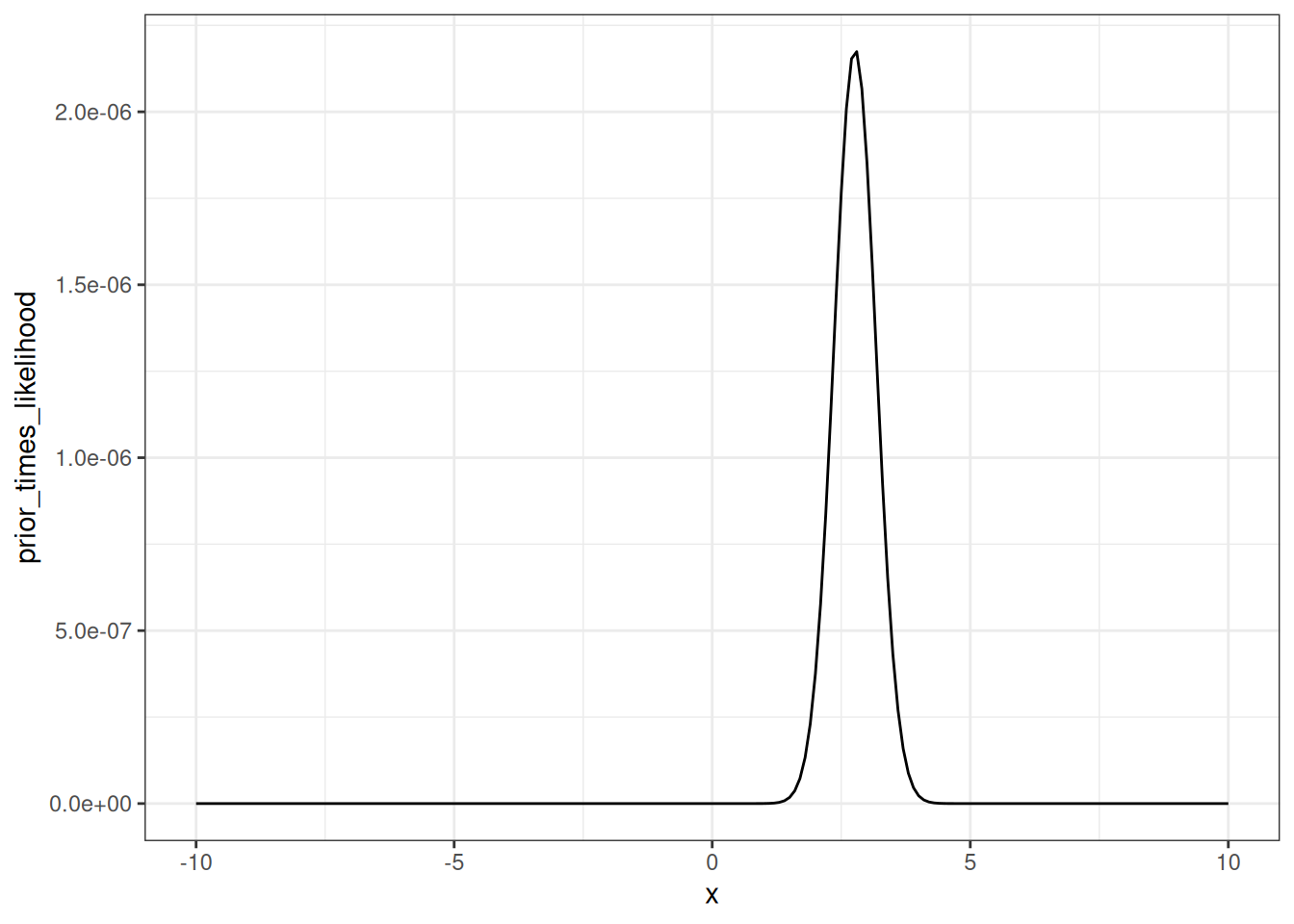
But from Bayes rule, we can rescale the prior * likelihood by the area under the curve to convert to a probability density function.
area_under_curve <- sum(prior_times_likelihood * delta_x)  #sum(Width * Height) = total probability of the data given all possible values of the parameter
normalized_posterior <- prior_times_likelihood / area_under_curve
The probability of the data is (i.e., the area under likelihood * prior curve): 2.2325827^{-6}
Now we can visualize the rescaled likelihood (remember that the un-scaled likelihood was used in the calculations), the prior, and the normalized posterior.
Figure 14.8 shows how the posterior is a blend of the prior and the likelihood.
tibble(x = x,
       prior = density_prior,
       likelihood = density_likelihood_rescaled,
       normalized_posterior = normalized_posterior) %>%
  pivot_longer(cols = -x, names_to = "distribution", values_to = "density") %>%
  mutate(distribution = factor(distribution)) %>%
  ggplot(aes(x = x, y = density, color = distribution)) +
  geom_line()  +
  theme_bw()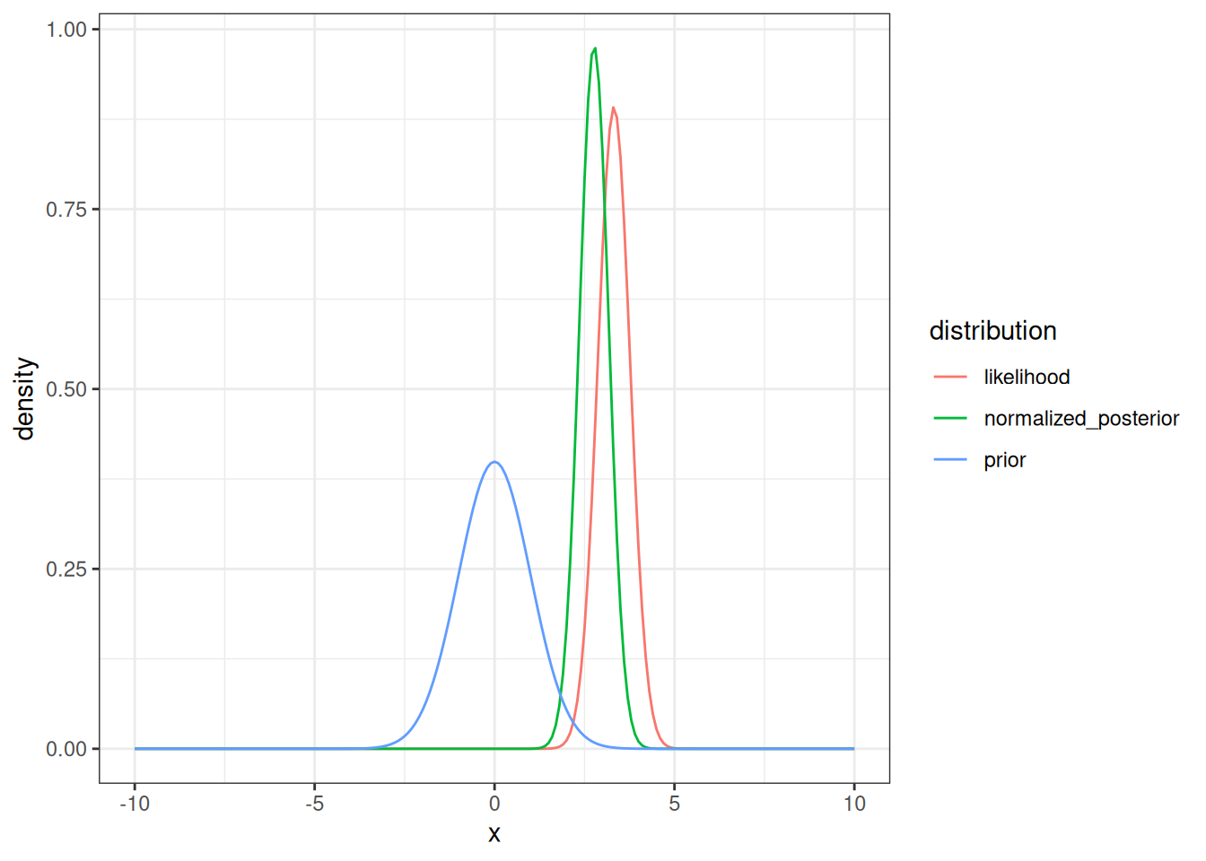
Here is a function that will allow us to explore how the posterior is sensitive to the likelihood and the prior.
explore_senstivity <- function(num_data_points, mean_data, sd_data, mean_prior, sd_prior, title){
new_data <- rnorm(num_data_points, mean_data, sd_data)
delta_x <- 0.1
x <- seq(-15,15, delta_x)
negative_log_likelihood <- rep(NA,length(x))
#DATA MODEL
for(i in 1:length(x)){
#Process model is that mean = x
negative_log_likelihood[i] <- -sum(dnorm(new_data, mean = x[i], sd = 1, log = TRUE))
}
density_likelihood <- exp(-negative_log_likelihood)
likelihood_area_under_curve <- sum(density_likelihood * delta_x) #Width * Height
density_likelihood_rescaled <- density_likelihood/likelihood_area_under_curve
#Prior
density_prior <- dnorm(x, mean = mean_prior, sd = sd_prior)
#Prior x Likelihood
prior_times_likelihood <- density_prior * density_likelihood
area_under_curve <- sum(prior_times_likelihood * delta_x) #Width * Height
normalized_posterior <- prior_times_likelihood / area_under_curve
p <- tibble(x = x,
prior = density_prior,
likelihood = density_likelihood_rescaled,
normalized_posterior = normalized_posterior) %>%
pivot_longer(cols = -x, names_to = "distribution", values_to = "density") %>%
mutate(distribution = factor(distribution)) %>%
ggplot(aes(x = x, y = density, color = distribution)) +
geom_line() +
labs(title = title) +
theme_bw()
return(p)
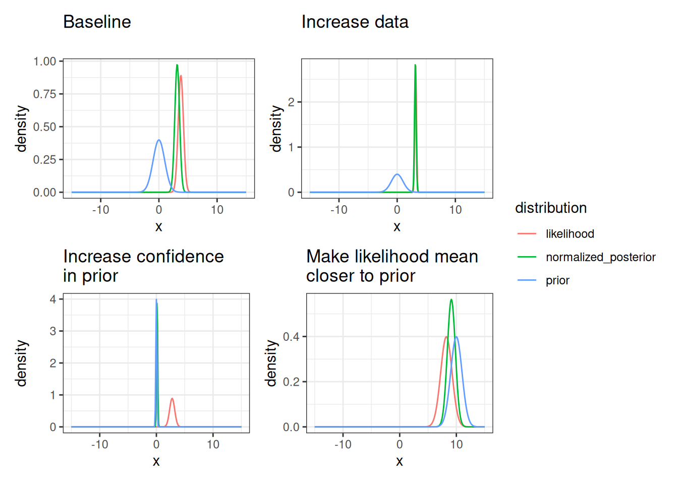
}Now we can explore how the posterior is sensitive to 1) prior sd (i.e., confidence in the prior) 2) the number of data points used in the likelihood (how does increasing the number of data points influence the posterior) the prior mean 3) the mean of the data used in the likelihood (how different is it than the prior?)
#Baseline
p1 <- explore_senstivity(num_data_points = 5,
                         mean_data = 3,
                         sd_data = 2,
                         mean_prior = 0,
                         sd_prior = 1.0,
                         title = "Baseline\n")

#Increase confidence in prior
p2 <- explore_senstivity(num_data_points = 5,
                         mean_data = 3,
                         sd_data = 2,
                         mean_prior = 0,
                         sd_prior = 0.1,
                         title = "Increase confidence\nin prior")

#Increase the number of data points
p3 <- explore_senstivity(num_data_points = 50,
                         mean_data = 3,
                         sd_data = 2,
                         mean_prior = 0,
                         sd_prior = 1.0,
                         title = "Increase data\n")

#Make likelihood mean closer to the prior
p4 <- explore_senstivity(num_data_points = 5,
                         mean_data = 0,
                         sd_data = 2,
                         mean_prior = 0,
                         sd_prior = 1.0,
                         title = "Make likelihood mean\ncloser to prior")


p4 <- explore_senstivity(num_data_points = 1,
                        mean_data = 10,
                        sd_data = 1.0,
                        mean_prior = 10,
                        sd_prior = 1.0,
                        title = "Make likelihood mean\ncloser to prior")
Figure 14.9 shows the sensitivity of the posterior to assumptions of the prior and the data.
Just like we extended the likelihood analysis to the non-linear example, we can do the same for the Bayesian analysis.
First, create a data set using the Michaelis-Menten function from the likelihood exercise. Here, instead of fitting both parameters, we only fit one parameter (the maximum or saturating value) called par1. In the chunk below we set the number of data points, the true value for par1, and the standard deviation of the data.
num_data_points <- 10
par1_true <- 3
sd_data <- 0.5
x <- runif(num_data_points, 0, 10)
par_true <- c(par1_true, 0.5)
y_true <- par_true[1] * (x / (x + par_true[2]))
y <- rnorm(length(y_true), mean = y_true, sd = sd_data)plot(x, y, ylim = c(0, par1_true + 2))
Now we can define the prior. We think the prior is normally distributed with a mean and sd defined below
mean_prior <- 1.0
sd_prior <- 0.5
Here is the manual calculation of the likelihood and the prior. We combine the results into a data frame for visualization.
delta_par1 <- 0.1
par1 <- seq(-3,10, delta_par1)
negative_log_likelihood <- rep(NA,length(par1))
for(i in 1:length(par1)){
  #Process model
  pred <- par1[i] * (x / (x + par_true[2]))
  #Data model
  negative_log_likelihood[i] <- -sum(dnorm(y, mean = pred, sd = sd_data, log = TRUE))
}

density_likelihood <- exp(-negative_log_likelihood)
likelihood_area_under_curve <- sum(density_likelihood * delta_par1) #Width * Height
density_likelihood_rescaled <- density_likelihood/likelihood_area_under_curve

#Priors
density_prior <- dnorm(par1, mean = mean_prior, sd = sd_prior)
prior_times_likelihood <- density_prior * density_likelihood
area_under_curve <- sum(prior_times_likelihood * delta_par1) #Width * Height
normalized_posterior <- prior_times_likelihood / area_under_curvetibble(par1 = par1,
prior = density_prior,
likelihood = density_likelihood_rescaled,
normalized_posterior = normalized_posterior) %>%
pivot_longer(cols = -par1, names_to = "distribution", values_to = "density") %>%
mutate(distribution = factor(distribution)) %>%
ggplot(aes(x = par1, y = density, color = distribution)) +
geom_line() +
theme_bw()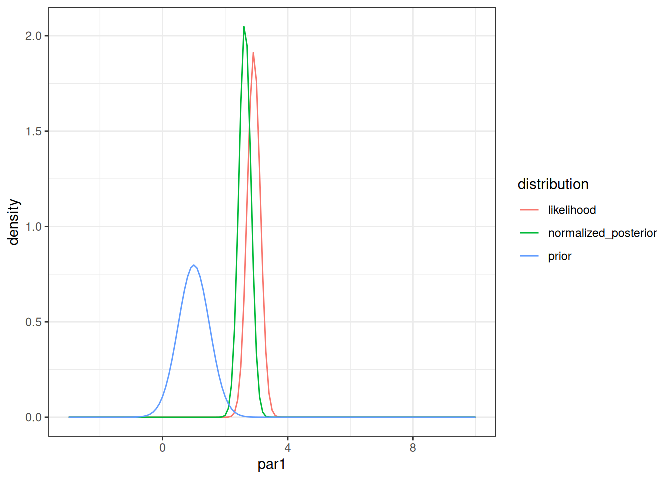
Now we can look at how our prior and posterior distributions influence the shape of the process model curve (M-M). For illustration, the figure below shows the M-M curve using the most likely value from the prior, the most likely value if we just looked at the likelihood, and the most likely value from the posterior.
par1_mle <- par1[which.max(density_likelihood)]
par1_post <- par1[which.max(normalized_posterior)]

d <- tibble(x = seq(0,10, 0.1),
            prior = mean_prior * (x / (x + par_true[2])),
            likelihood = par1_mle * (x / (x + par_true[2])),
            posterior = par1_post * (x / (x + par_true[2]))) %>%
  pivot_longer(cols = -x, names_to = "distribution", values_to = "prediction") %>%
mutate(distribution = factor(distribution))ggplot(d, aes(x = x, y = prediction, col = distribution)) +
geom_line() +
labs(y = "M-M model prediction (process model)") +
theme_bw()
14.2 Solving a Bayesian model
The example above is designed to build an intuition for how a Bayesian analysis works but is not how the parameters in a Bayesian model are estimated in practice. For one thing, if there are multiple parameters being estimated, it is very hard to estimate the area under the curve. Second, the area is very very small if there are many data points (so small that the computer can’t hold it well).
There are two common methods for estimating posterior distributions that involve numerical computation. Both methods involve randomly sampling from an unknown posterior distribution and saving the samples. The sequence of saved samples of the parameters is called a Markov chain Monte Carlo (MCMC). The distribution of parameter values in the MCMC chain is your posterior distribution.
The first is called Gibbs sampling and is used when you know the probability distribution type for the posterior but not the parameter values of the distribution. For example, if your prior is normally distributed and your likelihood is normally distributed then you know (from math that others have already done for you) that the posterior is normally distributed. Therefore, you can randomly draw from that distribution to build your MCMC chain that generates your posterior distribution. We will not go over this in detail but know that this method will give you an answer quicker but requires you (or the software you are using) to know that your prior and likelihood are conjunct (i.e., someone else has worked out that the posterior always has a certain PDF if the prior and likelihood are of certain PDF - see pages 86-89 and Table A3 in Hobbs and Hooten).
The second is called MCMC Metropolis-Hastings (MCMC-MH) and is a rejection sampling method. In this case, you don’t know the form of the posterior. Basically, the MCMC-MH is the following
Create a vector that has a length equal to the total number of iterations you want to have in your MCMC chain. Set the first value of the vector to your parameter starting point.
randomly choose a new parameter value based on the previous parameter value in the MCMC chain (called a proposal). For example (where i is the current iteration in your MCMC chain):
par_proposed <- rnorm(1, mean = par[i - 1], sd = jump), wherejumpis the standard deviation that governs how far you want the proposed parameter to potentially be from the previous parameter.use this proposed parameter in your likelihood and prior calculations and multiply the likelihood * prior (i.e., the numerator in Bayes formula). Save this as the proposed probability(
prob_proposed)Take the ratio of the proposed probability to the previous probability (also called the current probability;
prob_current). call thisprob_proposedRandomly select a number between 0 and 1. Call this
zIf
prob_proposedfrom Step 3 is greater thanzfrom Step 4 then save the proposed parameter for that iteration of MCMC chain. If it is less, then assign the previous parameter value for that iteration of the MCMC chain. As a result of Step 5:
- All parameters that improve the probability will have
prob_proposed/prob_current> 1. Therefore all improvements will be accepted since z (by definition in Step 4) can never be greater than 1. - Worse parameters where
prob_proposed/prob_current< 1, will be accepted in proportion to how worse they are. For example ifprob_proposed/prob_current= 0.9, 90% of the time z will be less the 0.90 so the worse parameters that are worse by 10% will be accepted 90% of the time. Ifprob_proposed/prob_current= 0.01 (i.e., the new parameters are much worse), only 1% of the time will z be less than 0.01. Therefore it is possible but not common to save these worse parameters. As a result, the MCMC-MH approach explores the full distribution by spending more time at more likely parameter values. This is different than maximum likelihood optimization methods likeoptimthat only save parameters that are better than the previous (thus finding the peak of the mountain rather than the shape of the mountain). The MCMC-HM approach requires taking a lot of samples so that it spends some time at very unlikely values - a necessity for estimating the tails of a distribution. - You want to accept ~40% percent of all proposed parameter values. If your jump parameter from #1 is too large, you won’t be able to explore the area around the most likely values (i.e., you won’t get a lot of
prob_proposed/prob_currentvalues near 1). If your jump parameter from #1 is too small, you won’t be able to explore the tails of the distribution (i.e., you won’t get a lot ofprob_proposed/prob_currentvalues near 0 that have a random chance of being accepted).
Note: There is a step that is ignored here that just confuses at this stage. Your proposal distribution in #1 doesn’t have to be normal, which is symmetric (i.e., your probability of jumping from a value of X to Y is the same as jumping from Y to X). There is an adjustment for non-symmetric proposals that is on page 71 in Dietze and page 158 in Hobbs and Hooten.
Here is an example of the MCMC-MH method:
(Note: the example below should use logged probability densities for numerical reasons but use the non-logged densities so that the method is clearer. The example in the assignment uses logged densities).
Set up data (same as above)
num_data_points <- 10
par1_true <- 3
sd_data <- 0.5
x <- runif(num_data_points, 0, 10)
par_true <- c(par1_true, 0.5)
y_true <- par_true[1] * (x / (x + par_true[2]))
y <- rnorm(length(y_true), mean = y_true, sd = sd_data)plot(x, y, ylim = c(0, par1_true + 2))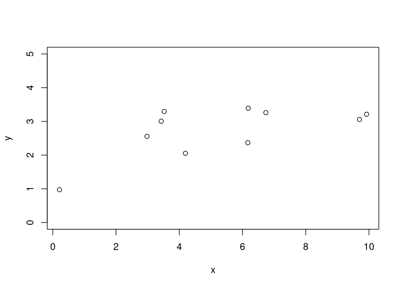
Run MCMC-MH
#Initialize chain
num_iter <- 1000
pars <- array(NA, dim = c(num_iter))
pars[1] <- 2
log_prob_current <- -10000000000
prob_current <- exp(log_prob_current)
jump <- 0.8

mean_prior <- 1.0
sd_prior <- 0.5

accept <- rep(NA,num_iter)
accept[1] <- 1

for(i in 2:num_iter){

  #Randomly select new parameter values
  proposed_pars <- rnorm(1, pars[i - 1], jump)


  #PRIORS: how likely is the proposed value given the prior distribution?
  prior <- dnorm(proposed_pars, mean = mean_prior, sd = sd_prior)

  #PROCESS MODEL: Use new parameter values in the process model
  pred <- proposed_pars * (x / (x + par_true[2]))

  #DATA MODEL: how likely is the data given the proposed parameter?
  #We are multiplying here
  likelihood <- prod(dnorm(y, mean = pred, sd = sd_data))

  #Combine the prior and likelihood
  #remember that you multiply probabilities which means you can add log(probability)
  prob_proposed <- prior * likelihood

  z <- (prob_proposed/prob_current)

  #Now pick a random number between 0 and 1
  r <- runif(1, 0, 1)

  #If z > r then accept the new parameters
  #Note: this will always happen if the new parameters are more likely than
  #the old parameters z > 1 means than z is always > r no matter what value of
  #r is chosen.  However, it will accept worse parameter sets (P_new is less
  #likely then P_old - i.e., z < 1) in proportion to how much worse it is
  #For example: if z = 0.9 and then any random number drawn by `runif` that is
  #less than 0.90 will result in accepting the worse values (i.e., the slightly
  #worse values will be accepted a lot of the time).  In contrast, if z = 0.01
  #(i.e., the new parameters are much much worse), then they can still be accepted
  #but much more rarely because random r values of < 0.1 occur more rarely
  #print(c(pars[i - 1], proposed_pars, z, r))
  if(z > r){
    accept[i] <- 1
    pars[i] <- proposed_pars
    prob_current <- prob_proposed
  }else{
    accept[i] <- 0
    pars[i] <- pars[i - 1]
    prob_current <- prob_current #this calculation isn't necessary but is here to show you the logic
  }
}
The pars variable is our MCMC chain estimating the posterior distribution. We can visualize it in two ways. The first is with the iteration number on the x-axis. The second is a histogram. A chain that is ready for analysis will have a constant mean and variance. The variance is important because it is the exploration of the posterior distribution. The histogram shows the posterior distribution.
d <- tibble(iter = 1:num_iter,
       par1 = pars)

p1 <-  ggplot(d, aes(x = iter, y = par1)) +
  geom_line()  +
  theme_bw()

p2 <- ggplot(d, aes(x = par1)) +
  geom_histogram() +
  theme_bw()

p1 | p2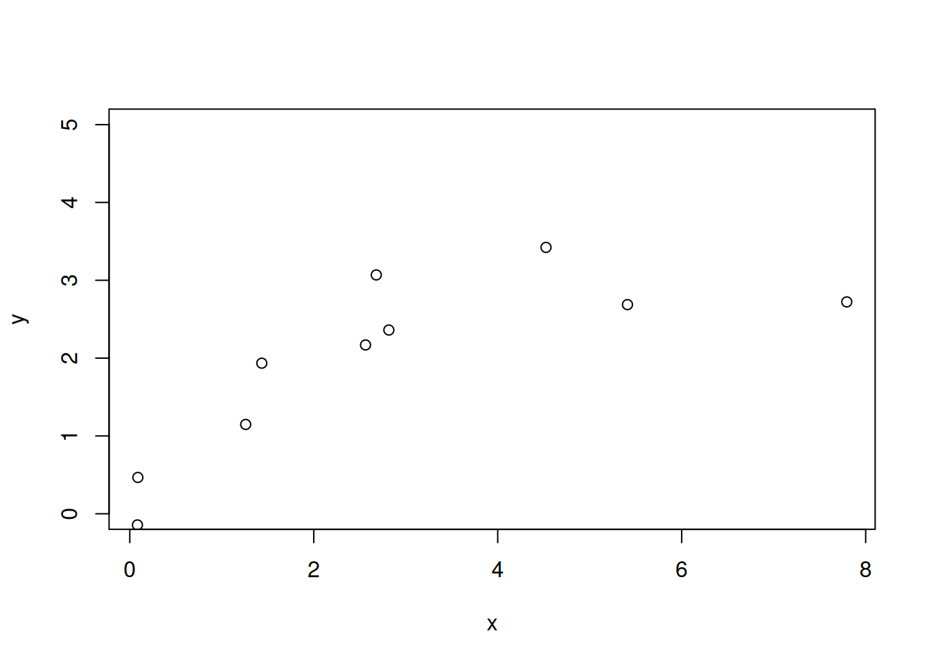
You should notice that the chain starts at 2 before moving to a mean of 3. The starting value of 2 was arbitrary. Since it was far from 3, the proposed new parameter values often resulted in improvements and accepting more likely values. As a result, the chain moves to the part with a mean of 3 and constant variance (i.e., where the chain has converged). This transition from the starting value to the point where the chain has converged should be discarded. We call this the “burn-in”. Here are the same plots with the burn-in removed.
nburn <- 100
d_burn <- tibble(iter = nburn:num_iter,
       par1 = pars[nburn:num_iter])
p1 <- ggplot(d_burn, aes(x = iter, y = par1)) +
geom_line() +
theme_bw()
p2 <- ggplot(d_burn, aes(x = par1)) +
geom_histogram() +
theme_bw()
p1 | p2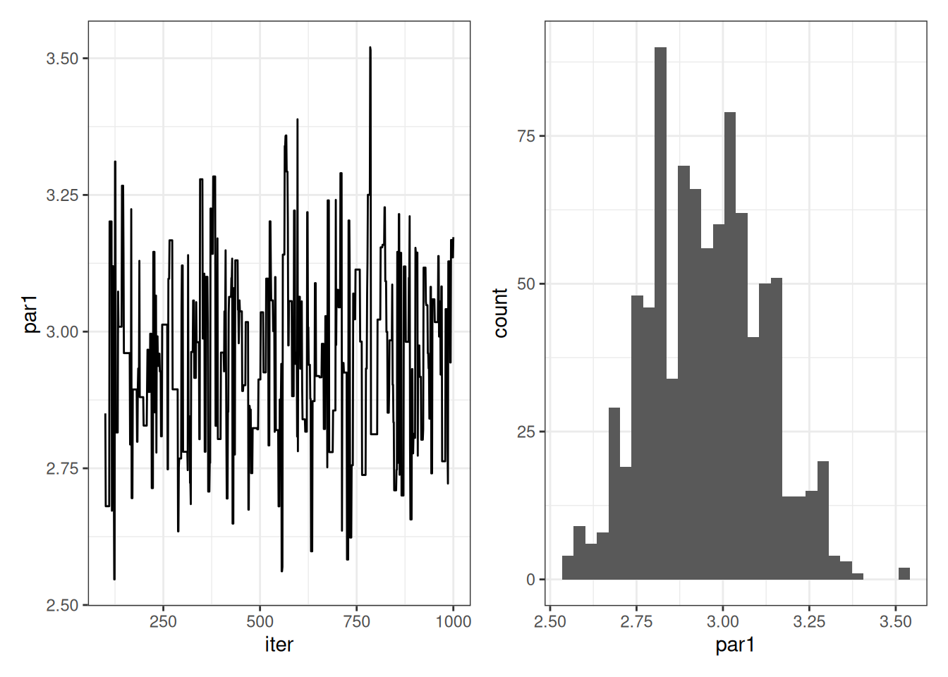
Now you can analyze the chain to explore the posterior distribution
par_post_burn <- pars[nburn:num_iter]

#Mean
mean(par_post_burn)
[1] 2.952403#sd
sd(par_post_burn)[1] 0.1653424#Quantiles
quantile(par_post_burn, c(0.025, 0.5,0.975)) 2.5% 50% 97.5%
2.652697 2.960757 3.281253 Finally, you can sample from the posterior distribution just like you would sample from a random variable using the rnorm, rexp, rlnorm, etc. function. The key is to randomly select an iteration (num_sample = 1) or a set of samples (if num_sample > 0) with replacement (replace = TRUE; i.e., an iteration could be randomly selected multiple times).
num_samples <- 100
sample_index <- sample(x = 1:length(par_post_burn), size = num_samples, replace = TRUE)
random_draws <- par_post_burn[sample_index]hist(random_draws)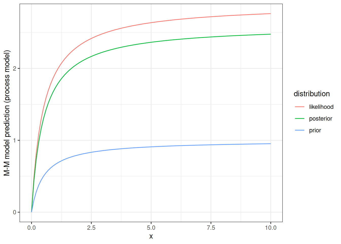
14.3 Predictive posterior distributions
Finally, we can use the idea of randomly drawing from the posterior to develop predictions from the posterior. This is just like the Logistic growth module where you randomly sampled from the parameter uncertainty and used the random samples in the logistic equation.
Here we are calculating two things 1) pred_posterior_mean just has uncertainty in the M-M model parameter. Think about this as generating uncertainty around the mean prediction at each value of x. 2) y_posterior is the prediction of an observation. Therefore, you take the value from #1 and add the uncertainty in the observations from sd_data that was set above. This is your predictive or forecast uncertainty.
num_samples <- 1000
x_new <- x
pred_posterior_mean <- matrix(NA, num_samples, length(x_new))   # storage for all simulations
y_posterior <- matrix(NA, num_samples, length(x_new))

for(i in 1:num_samples){
  sample_index <- sample(x = 1:length(pars), size = 1, replace = TRUE)
  pred_posterior_mean[i, ] <- pars[sample_index] * (x_new / (x_new + par_true[2]))
  y_posterior[i, ] <- rnorm(length(x_new), pred_posterior_mean[i, ], sd = sd_data)

}
n.stats.y <- apply(y_posterior, 2, quantile, c(0.025, 0.5, 0.975))
n.stats.y.mean <- apply(y_posterior, 2, mean)

n.stats.mean <- apply(pred_posterior_mean, 2, quantile, c(0.025, 0.5, 0.975))

d <- tibble(x = x_new,
            median = n.stats.y.mean,
            lower95_y = n.stats.y[1, ],
            upper95_y = n.stats.y[3, ],
            lower95_mean = n.stats.mean[1, ],
            upper95_mean = n.stats.mean[3, ],
obs = y)ggplot(d, aes(x = x)) +
geom_ribbon(aes(ymin = lower95_y, ymax = upper95_y), fill = "lightblue", alpha = 0.5) +
geom_ribbon(aes(ymin = lower95_mean, ymax = upper95_mean), fill = "pink", alpha = 0.5) +
geom_line(aes(y = median)) +
geom_point(aes(y = obs)) +
labs(y = "M-M Prediction") +
theme_bw()
14.4 Important considerations
14.4.1 Joint vs marginal distributions
If you have multiple parameters in your MCMC chain, you randomly draw posterior_sample_indices and use values for all the parameters at that iteration. By doing this you are representing the joint distribution of the parameter - e.g., if parameter 1 is high, parameter 2 is always low. If you select posterior_sample_indices for each parameter, you break the correlations of parameters that the MCMC method estimated and, as a result, overestimate the uncertainty.
14.4.2 Identifiability
Imagine you have a model that predicts water temperature as a linear function of air temperature but uses the following equation:
water temperature = m + a * b * air temperature
In this toy example, the slope has been separated into two parameters (a and b). As a result, you can get the same value for a slope with a large value a and a small value for b as when you have a small value for a and a large value for b. Consequentially it is impossible to find a value for either a or b and these parameters are unidentifiable. If you collapse the a*b down into a single parameter (m) then that parameter is identifiable.
In an ecosystem example, we often use net fluxes (like net ecosystem exchange) to calibrate models. Since NEE is the net of respiration and photosynthesis, the same NEE can emerge from a system with large values for respiration and photosynthesis as a system with small values for respiration and photosynthesis. Therefore the parameters that govern respiration and photosynthesis are not identifiable using only NEE data for parameter estimation.
Identifiability issues can be addressed by 1) adding additional data sources for parameter estimation. For example, in the next chapter, we use NEE and LAI in the calibration. The LAI data helps separate the low production from the high production system because a lower production system can not be associated with high LAI values in the model. 2) by using “stronger” priors that have distributions with less spread (see below) or 3) by modifying the equation(s) of the model to reduce the trade-off in parameters.
14.4.3 Data leakage
Data that contributed to the prior distribution can be me used in the likelihood (data leaking from the prior to posterior). This will result in artificial re-enforcement of the prior and will give artificially large confidence in the posterior. Similarly, data that you collected that will be used in the likelihood can not be used to develop the prior.
You can use data that you will use in your likelihood calculation to involve the starting point of your MCMC chain. In some cases, a maximum likelihood fit of your model, like in Chapter 13, will yield starting points that are very close mean of the posterior (just without the uncertainty estimation). By starting your MCMC chain at these maximum likelihood estimates for the parameters, you will reduce the burn-in iterations and increase the computational efficiency of your Bayesian analysis. This is not data leakage.
14.5 Priors
Informed, strong vs. uninformed, vague, weak
The parameters of the distribution determine how informed the prior is. For example, a normal distribution with a mean = 0 and sd = 0.1 is much more informed than one with the sd = 1000 (the latter has similar probability densities across a large range of parameter values). It is also important to consider the range of support in a distribution. For example, a normal distribution has non-zero densities for parameter values from -infinity to +infinity. Therefore the prior density for a parameter value will never be 0 (thus resulting in the prior * likelihood = 0, and the MCMC never accepting that parameter value). In contrast, a uniform distribution has hard bounds that are user-provided. If the prior is uniform from 0 to 1, then no parameter values less than 0 or greater than 1 will be considered even if the data supports these values. Other probability distributions have embedded bounds. For example, the log-normal distribution can have values less than 0. Overall, hard bounds can be desired because of biophysical constraints on the parameter (e.g., a rate parameter or a proportion parameter can’t be negative).
In some cases, they are so informed that you assume they are a fixed value. Justification for the parameter value choice when fixing a parameter or using a strong prior.
Remember that the priors are for specific parameters in the model. The information used to develop informed priors must come from comparable information about the same parameter.
Literature review
Databases
Expert options/survey
14.5.1 Prior key points
You may want to consider informed priors if
There are known issues with parameter identifiability in your model
The parameter is a physical constant (like gravity constant)
There is considerable prior research on a parameter
There are physical constraints to a parameter (e.g., it can’t be a negative value)
You may consider using informed priors if there is a history of using a set of parameter values in previous applications of the model. In this case, be aware of zombie parameters, that is parameters whose values appear from the literature to be known because everyone uses it, but are in fact a relic of a modeler’s decision in the past that has carried through many model applications without being closely examined. The parameter may be less certain than the literature indicates.
You may want to consider uninformed priors if
- You need a prior for the parameter but do not have any information about it.
- There is a desire to have the analysis reflect the data only
14.6 Additional Bayesian topics
This chapter is an introduction to the concepts and numerical techniques used in Bayesian analysis. There are more advanced topics that may be of interest but are not covered here. These include:
State-space modeling: state-space models are used to estimate process uncertainty for dynamic models like the forest model in Chapter 16. When estimating process uncertainty using a state-space model, the uncertainty represents the uncertainty that accumulates between time steps in the model.
Hierarchical models: Hierarchical models are used when you want a parameter to vary over time and space but don’t want to estimate unique parameters for every space and time point. Hierarchical models allow for you to estimate a “global” parameter distribution whereby the individual parameters at a site or a point in time are samples from the global distribution. Hierarchical models allow information from one site to help inform parameter values for another site while considering them independent.
Packages for posterior estimation: Many packages exist to estimate posteriors in Bayesian models that differ in their algorithms, capacities for complex applications, and available documentation. These include Stan, JAGS, Nimble, and greta. All packages can solve simple Bayesian problems like the M-M example above. Packages have different strengths for solving more complex problems. Some are also more well-suited for use with custom functions and dynamic models like the forest model in this book.
More robust algorithms for estimating posteriors and the use of conjecture priors to speed posterior estimation.
14.7 Reading
14.8 Problem Set
The problem set is located in bayesian_problem_set.qmd in https://github.com/frec-5174/book-problem-sets. You can fork the repository or copy the code into your own quarto document