site <- "OSBS"
ens_members <- 100
sim_dates <- seq(Sys.Date() - 365*2, Sys.Date() - 2, by = "1 day")
#sim_dates <- seq(as_date("2020-09-30"), as_date("2025-12-15") - lubridate::days(2), by = "1 day")20 Applying to data assimilation to process model
In this chapter, we apply the particle filter that was introduced in Chapter 15 to the forest process model. We will use an ensemble of 100 particles and assimilate the last two years of data.
20.1 Prep data
Get the historical weather for the site
inputs <- get_historical_met(site = site, sim_dates, use_mean = FALSE)
inputs_ensemble <- assign_met_ensembles(inputs, ens_members)
Set the constant parameters (we will fit two parameters using the particle filter below)
params <- list()
params$alpha <- rep(0.02, ens_members)
params$SLA <- rep(4.74, ens_members)
params$leaf_frac <- rep(0.315, ens_members)
params$Ra_frac <- rep(0.5, ens_members)
params$Rbasal <- rep(0.002, ens_members)
params$Q10 <- rep(2.1, ens_members)
params$litterfall_rate <- rep(1/(2.0*365), ens_members) #Two year leaf lifespan
params$litterfall_start <- rep(200, ens_members)
params$litterfall_length<- rep(70, ens_members)
params$mortality <- rep(0.00015, ens_members) #Wood lives about 18 years on average (all trees, branches, roots, course roots)
params$sigma.leaf <- rep(0.1, ens_members) #0.01
params$sigma.wood <- rep(0.1, ens_members) #0.01 ## wood biomass
params$sigma.soil <- rep(0.1, ens_members)# 0.01
params <- as.data.frame(params)
Read in the observational data and use the first data in the simulation period as the initial condition.
obs <- read_csv("data/site_carbon_data.csv", show_col_types = FALSE)
state_init <- rep(NA, 3)

state_init[1] <- obs |>
  filter(variable == "lai",
         datetime %in% sim_dates) |>
  na.omit() |>
  slice(1) |>
  mutate(observation = observation / (mean(params$SLA) * 0.1)) |>
  pull(observation)

state_init[2] <- obs |>
  filter(variable == "wood",
         datetime %in% sim_dates) |>
  na.omit() |>
  slice(1) |>
  pull(observation)

state_init[3] <- obs |>
  filter(variable == "som") |>
  na.omit() |>
  slice(1) |>
  pull(observation)
Assign the initial conditions to the first time-step of the simulation
#Set initial conditions
forecast <- array(NA, dim = c(length(sim_dates), ens_members, 12)) #12 is the number of outputs
forecast[1, , 1] <- state_init[1]
forecast[1, , 2] <- state_init[2]
forecast[1, , 3] <- state_init[3]

wt <- array(1, dim = c(length(sim_dates), ens_members))
Read in the parameter chain from Chapter 19. We sample from the chain to get the initial starting distribution for the particle filter. Importantly, the parameter has to be sampled together to preserve the correlation between them. In our example, assume the litterfall_start is constant at the calibrated mean.
fit_params_table <- read_csv("data/saved_parameter_chain.csv", show_col_types = FALSE) |>
  pivot_wider(names_from = parameter, values_from = value)

num_pars <- 2
fit_params <- array(NA, dim = c(length(sim_dates) ,ens_members , num_pars))
samples <- sample(1:nrow(fit_params_table), size = ens_members, replace = TRUE)
fit_params[1, , 1] <- fit_params_table$alpha[samples]
fit_params[1, , 2] <- fit_params_table$Rbasal[samples]
params$litterfall_start <- mean(fit_params_table$litterfall_start, na.rm = TRUE)
20.2 Run the particle filter
In the particle filter, we perturb the parameter values slightly to prevent them from collapsing to a single value.
for(t in 2:length(sim_dates)){

  fit_params[t, , 1] <- rnorm(ens_members, fit_params[t-1, ,1], sd = 0.0005)
  fit_params[t, , 2] <- rnorm(ens_members, fit_params[t-1, ,2], sd = 0.00005)

  params$alpha  <- fit_params[t, , 1]
  params$Rbasal  <- fit_params[t, , 2]

  forecast[t, , ]  <- forest_model(t,
                                   states = matrix(forecast[t-1 , , 1:3], nrow = ens_members) ,
                                   parms = params,
                                   inputs = matrix(inputs_ensemble[t , , ], nrow = ens_members))

  curr_obs <- obs |>
    filter(datetime == sim_dates[t],
           variable %in% c("nee","lai","wood"))

  if(nrow(curr_obs) > 0){

    forecast_df <- output_to_df(forecast[t, , ], sim_dates[t], sim_name = "particle_filter")


    combined_output_obs <- combine_model_obs(forecast_df,
                                             obs = curr_obs,
                                             variables = c("lai", "wood", "som", "nee"),
                                             sds = c(0.1, 1, 20, 0.005))

    likelihood <- rep(0, ens_members)
    for(ens in 1:ens_members){

      curr_ens <- combined_output_obs |>
        filter(ensemble == ens)

      likelihood[ens] <- exp(sum(dnorm(x =  curr_ens$observation,
                                       mean = curr_ens$prediction,
                                       sd = curr_ens$sds, log = TRUE)))
    }

    wt[t, ] <- likelihood * wt[t-1, ]

    wt_norm <-  wt[t, ]/sum(wt[t, ])
    Neff = 1/sum(wt_norm^2)

    if(Neff < ens_members/2){
      ## resample ensemble members in proportion to their weight
      resample_index <- sample(1:ens_members, ens_members, replace = TRUE, prob = wt_norm )
      forecast[t, , ] <- as.matrix(forecast[t, resample_index, 1:12])  ## update state
      fit_params[t, , ] <- as.matrix(fit_params[t, resample_index, ])
      wt[t, ] <- rep(1, ens_members)
    }
  }
}
Process the output and parameters into a data frame using the particle weights.
forecast_weighted <- array(NA, dim = c(length(sim_dates), ens_members, 12))
params_weighted <- array(NA, dim = c(length(sim_dates) ,ens_members , num_pars))
for(t in 1:length(sim_dates)){
  wt_norm <-  wt[t, ]/sum(wt[t, ])
  resample_index <- sample(1:ens_members, ens_members, replace = TRUE, prob = wt_norm )
  forecast_weighted[t, , ] <- forecast[t, resample_index, 1:12]
  params_weighted[t, , ] <- fit_params[t,resample_index, ]
}
output_df <- output_to_df(forecast_weighted, sim_dates, sim_name = "particle_filter")
parameter_df <- parameters_to_df(params_weighted, sim_dates, sim_name = "particle_filter", param_names = c("alpha","Rbasal"))
Visualize the simulation using the particle filter
obs_dates <- obs |>
  filter(variable == c("nee","lai", "wood")) |>
  pull(datetime)

output_df |>
  summarise(median = median(prediction),
            upper = quantile(prediction, 0.95, na.rm = TRUE),
            lower = quantile(prediction, 0.05, na.rm = TRUE), .by = c("datetime", "variable")) |>
  left_join(obs, by = c("datetime", "variable")) |>
  filter(variable %in% c("nee","wood","som","lai")) |>
  ggplot(aes(x = datetime)) +
  geom_ribbon(aes(ymin = upper, ymax = lower), alpha = 0.7) +
  geom_line(aes(y = median)) +
  geom_point(aes(y = observation), color = "red") +
  facet_wrap(~variable, scale = "free") +
  theme_bw()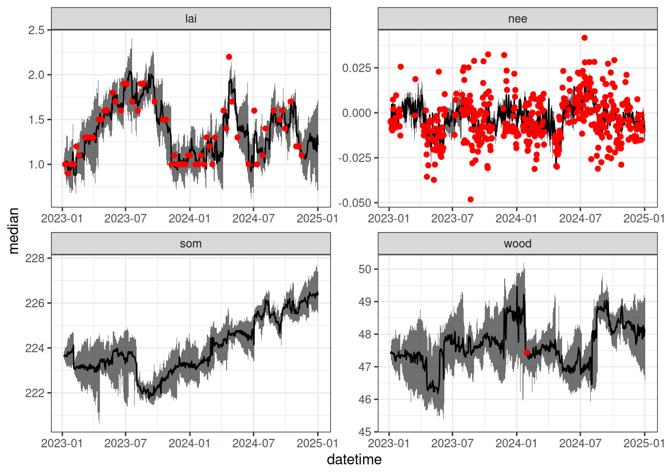
Visualize how the parameters changed over the simulation. You can see the distributions widening between observations and narrowing when an observation is assimilated.
parameter_df |>
  summarise(median = median(prediction),
            upper = quantile(prediction, 0.95, na.rm = TRUE),
            lower = quantile(prediction, 0.05, na.rm = TRUE), .by = c("datetime", "variable")) |>
  left_join(obs, by = c("datetime", "variable")) |>
  ggplot(aes(x = datetime)) +
  geom_ribbon(aes(ymin = upper, ymax = lower), alpha = 0.7) +
  geom_line(aes(y = median)) +
  facet_wrap(~variable, scale = "free") +
  theme_bw()
Combine the forecast, parameters, weights, simulation dates, and constant parameters into an object called analysis and save for use in Chapter 21
analysis <- list(forecast = forecast, fit_params = fit_params, wt = wt, sim_dates = sim_dates, params = params)
save(analysis, file = "data/PF_analysis_0.Rdata")