11  Evaluating forecasts

The fourth forecast-generation assignment will challenge you to analyze the automated forecasts you submitted as part of Chapter 10. The assignment uses the module in Freya Olsson’s tutorial that provides code to access the automatically scored forecasts. You will add code to your repository that generates plots.

Tutorial Rmarkdown

This chapter describes metrics for evaluating forecasts, including comparisons with simple baseline forecast models.

11.1 Scoring metrics

A scoring metric is a value used to evaluate how well a forecast compares with observations. Scores can then be compared among forecast models to evaluate relative performance. Typically, lower scores are better. Scoring metrics are also called “costs”.

11.2 Accuracy

The most basic score would be the difference between the forecast mean and the observation. However, there are a couple of issues with that score. First, forecasts below the observation will receive negative values and forecasts above will receive positive values, thus the lowest value is not the best. Second, it does not use any information from the forecast uncertainty in the evaluation. Metrics like absolute error (the absolute value of the difference between the forecast mean and the observation) and root-mean-squared error (RMSE) address the first issue but still do not account for uncertainty.

11.3 Precision

Is the variance in the forecast larger than an acceptable value? For example, if the uncertainty in a rain forecast ranges from a downpour to sunny, then the variance is too large to be useful, since one cannot make a specific decision based on the forecast (e.g., do you cancel the soccer game ahead of time?). One can also compare the variance of a forecast to that of a baseline variable from a simple model to see whether the spread is smaller, indicating a more informative forecast.

11.4 Accuracy + Precision

It is important to consider uncertainty because, intuitively, a forecast that has the correct mean but a large uncertainty (so it puts very little confidence on the observed value) should have a lower score than a forecast with a mean that is slightly off but with lower uncertainty (so it puts more confidence on the observed value). The Continuous Ranked Probability Score (CRPS) is one metric that evaluates the forecast distribution. Another is the ignorance score (also called the Good or the log score). The CRPS is described below.

11.4.1 Continuous Ranked Probability Score

Forecasts can be scored using the continuous ranked probability score (CRPS), a proper scoring rule for evaluating forecasts presented as distributions or ensembles (Gneiting and Raftery (2007)). The CRPS compares the forecast probability distribution to that of the validation observation and assigns a score based on both the accuracy and precision of the forecast. We will use the ‘crps_sample’ function from the scoringRules package in R to calculate the CRPS for each forecast.

CRPS is a calculation for each forecast-observation pair (e.g., a single datetime from a reference_datetime). CRPS can then be aggregated across all sites and forecast horizons to understand the aggregate performance.

Importantly, we use the CRPS convention, where zero is the lowest and best possible score; forecasts aim to achieve the lowest score. CPRS can also be expressed as a negative number with zero as the highest and best possible score (Gneiting and Raftery (2007)). The scoringRules package we use follows the 0 or greater convention.

library(scoringRules)
library(tidyverse)

11.4.1.1 Example of a CRPS calculation from an ensemble forecast

This section aims to provide an intuition for the CRPS metric.

First, create a random sample from a probability distribution. This is the “forecast” for a particular point in time. For simplicity, we will use a normal distribution with a mean of 8 and a standard deviation of 1

forecast <- rnorm(1000, mean = 8, sd = 2.0)

Second, we have our data point (i.e., the target) that we set to 8 as well.

observed <- 8

Now calculate using the crps_sample() function in the scoringRules package

library(scoringRules)
crps_sample(y = observed, dat = forecast)

[1] 0.4794483

11.4.1.2 Exploring the scoring surface

Now lets see how the CRPS changes as the mean and standard deviation of the forecasted distribution change

First, set vectors for the different mean and SD values we want to explore

forecast_mean <- seq(5, 11, 0.05)
forecast_sd <- seq(0.1,6, 0.05)

Second, use the same value for observed as above (8)

Now calculate the CRPS at each combination of forest mean and SD. We used crps_norm because we know the forecast is normally distributed

combined <- array(NA, dim = c(length(forecast_mean), length(forecast_sd)))
for(i in 1:length(forecast_mean)){
  for(j in 1:length(forecast_sd)){
    combined[i, j] <- crps_norm(y = observed, mean = forecast_mean[i], forecast_sd[j])
  }
}

Finally, the contour surface highlights the trade-off between the mean and standard deviation. Each isocline is the same CRPS score. Holding the mean constant at the observed value but increasing the uncertainty (increasing SD) results in a higher (worse) score (compare the green to the orange dot). Holding the SD constant but adding bias results in a higher (worse) score (compare the green to red dot).

contour(x = forecast_mean, y = forecast_sd, z = as.matrix(combined),nlevels = 20, xlab = "Forecast mean", ylab = "forecast standard deviation", main = "CPRS score at different forecasted mean and sd\nThe observation is at 8")
points(x = observed, y = 2, col = "green")
points(x = 6, y = 2, col = "red")
points(x = observed, y = 5, col = "orange")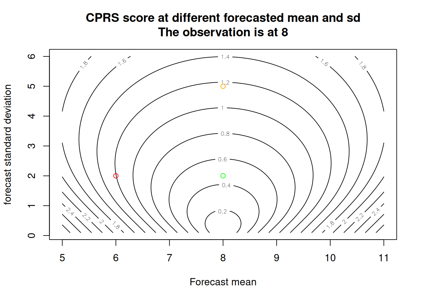

11.4.1.3 Calculating CRPS manually

The manual calculation of CRPS helps provide intuition for what the metric represents.

First, we are going to set the range of values (forecast or observation) to include in the calculation. In this case, we go 5 above and below the observed value. We will set dy to be 0.1 so we have values every 0.1.

dy <- 0.1
values_evaluated <- seq(observed - 5, observed + 5, dy)

We are going to convert our forecast to a cumulative density function using the ecdf function and then calculate the value of the cdf at each value we are exploring.

forecast_cdf_function <- ecdf(forecast)
forecast_cdf <- forecast_cdf_function(values_evaluated)

Next, calculate the cdf for the observation, where it is 0 if the observation is less than the observed value and 1 if it is greater.

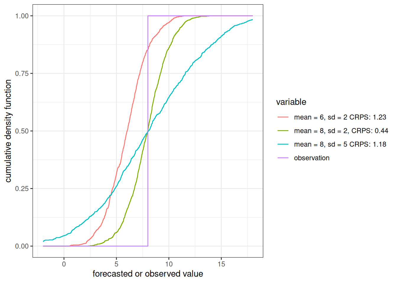
obs_cdf <- as.numeric((values_evaluated > observed))

Plot the two cdfs on the same plot

At a high level, CRPS is the area between the red and blue lines in the figure above. The area to the left of the observation is the error associated with the forecast, saying the observed value will be less than the actual observation. The area to the right of the observation is the error associated with the forecast, saying that the observed value is larger than the forecasted value.

By subtracting the observed cdf from the forecast cdf, we can calculate the difference between the two curves (square it to get the squared error).

error <- (forecast_cdf - obs_cdf)^2

Multiply by the squared difference (height) by dy (width) to get the area of each error bin.

cdf_diff_area <- error * dy

The sum of the areas in each bin is the crps

crps <- sum(cdf_diff_area)
crps

[1] 0.4794659

which is very similar to the answer from the scoringRules package. The difference is due to the size of dy. Smaller values of dy will yield results closer to those from scoringRules.

scoringRules::crps_sample(y = observed, dat = forecast)

[1] 0.4794483

You can compare different forecasts using the CDF to see how the areas differ

11.5 Dynamics

Add discussion of shadow time and correlation.

11.6 Skill scores

It is a best practice in forecasting to compare forecasts from more complex models with those from simple “naive” models to assess whether the additional complexity provides any gain in forecast capacity. Two common naive models are persistence and “climatology”.

The skill score compared a forecast model to a baseline model using the following equation

skill_score <- 1 - (mean_metric_baseline - mean_metric_forecast)/mean_metric_baseline

The mean_metric_baseline is the mean score for the baseline model. It can be RMSE, MAE, CPRS, etc. mean_metric_forecast is the same metric used to evaluate the forecast.

The skill score ranges from -Inf to 1, where values from -Inf to 0 are forecast models that perform worse than the baseline. Values from 0 to 1 are forecast models that improve on the baseline. A value of 1 means that the forecast model is perfect.

11.6.1 Example baseline models

Persistence forecasts that tomorrow will be the same as today, thereby capturing the system’s inertia. Uncertainty is added to a persistence forecast by simulating it as a random walk where each ensemble member has a random trajectory without any direction (so the mean of the forecast is still the previous day’s mean value). Persistence models perform well in systems with real-time observations because you know the current value, and in systems with high inertia (such as water temperatures at the bottom of a large lake).

persistence <- arrow::open_dataset("s3://anonymous@bio230014-bucket01/challenges/forecasts/bundled-summaries/project_id=neon4cast/duration=P1D/variable=temperature/model_id=persistenceRW?endpoint_override=sdsc.osn.xsede.org") |> 
  filter(site_id == "BARC",
         reference_date == as_date("2024-10-10")) |> 
  collect()

persistence |> 
  ggplot(aes(x = datetime)) +
  geom_ribbon(aes(ymin = quantile10, ymax = quantile90), color = "lightblue", fill = "lightblue", alpha = 0.7) +
  geom_line(aes(y = median)) +
  labs(y = "water temperature", x = "datetime", title = "NEON site: BARC") +
  theme_bw()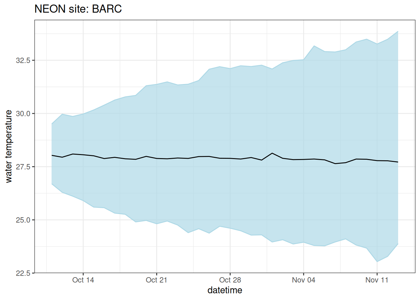

“Climatology” is the historical distribution of observations for the forecast days. In a seasonal system, we often represent this using the mean and standard deviation of historical data from the same day-of-year in the past. Less seasonal systems may represent it as the historical mean and standard deviation. I used climatology in quotes because the meteorological definition of climatology is 30 years, but most ecological systems don’t have 30 years of observations. We use the term “day-of-year mean” instead of climatology when forecasting systems with limited historical data. Climatology forecasts the system’s long-term behavior and its capacity to capture seasonal patterns.

climatology <- arrow::open_dataset("s3://anonymous@bio230014-bucket01/challenges/forecasts/bundled-summaries/project_id=neon4cast/duration=P1D/variable=temperature/model_id=climatology?endpoint_override=sdsc.osn.xsede.org") |> 
  filter(site_id == "BARC",
         reference_date == "2024-10-10") |> 
  collect()

climatology |> 
  ggplot(aes(x = datetime)) +
  geom_ribbon(aes(ymin = quantile10, ymax = quantile90), color = "lightblue", fill = "lightblue", alpha = 0.7) +
  geom_line(aes(y = median)) +
  labs(y = "water temperature", x = "datetime", title = "NEON site: BARC") +
  theme_bw()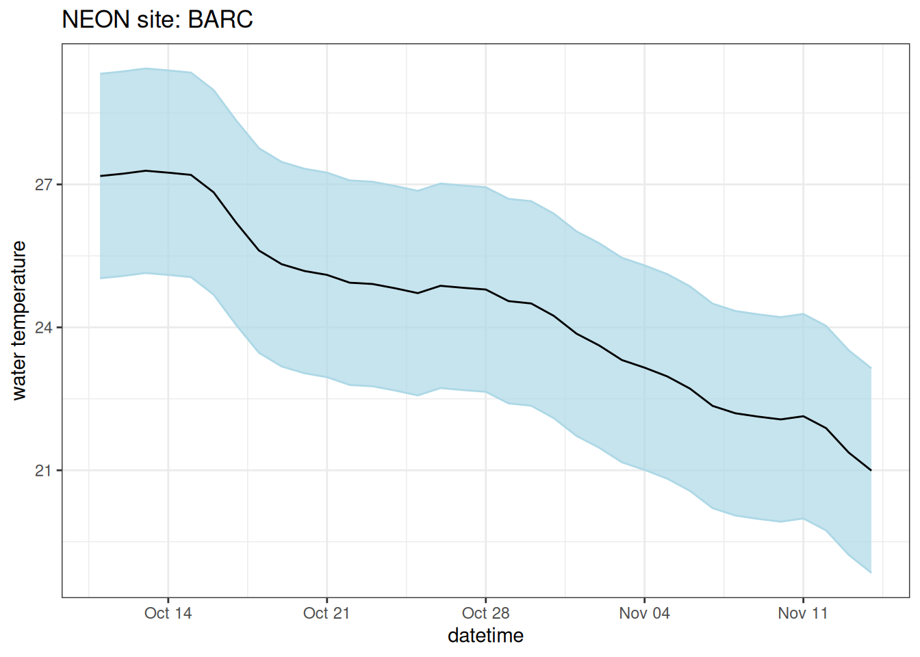

Both of these models are simple to calculate and include no “knowledge” of the system that might be embedded in more complex models.

11.6.2 Example skill score calculation

This example compares the skill of the climatology forecast to the persistence baseline

baseline_models <- arrow::open_dataset("s3://anonymous@bio230014-bucket01/challenges/scores/bundled-parquet/project_id=neon4cast/duration=P1D/variable=temperature?endpoint_override=sdsc.osn.xsede.org") |> 
  filter(site_id == "BARC",
         reference_datetime > lubridate::as_datetime("2024-09-01"),
         reference_datetime < lubridate::as_datetime("2024-10-31"),
         model_id %in% c("climatology", "persistenceRW")) |> 
  collect() 

skill_score <- baseline_models |> 
  mutate(horizon = as.numeric(datetime - reference_datetime)) |> 
  summarize(mean_crps = mean(crps, na.rm = TRUE), .by = c("model_id", "horizon")) |> 
  pivot_wider(names_from = model_id, values_from = mean_crps) |> 
  mutate(skill_score = 1 - (climatology/persistenceRW))

ggplot(skill_score, aes(x = horizon, y = skill_score)) +
  geom_line() +
  geom_hline(aes(yintercept = 0)) +
  labs(x = "Horizon (days in future)", y = "Skill score") +
  theme_bw() +
  annotate("text", label = "climatology is better", x = 15, y = 0.2) +
  annotate("text", label = "baseline (persistence) is better", x = 15, y = -0.2)

Warning: Removed 1 row containing missing values or values outside the scale range
(`geom_line()`).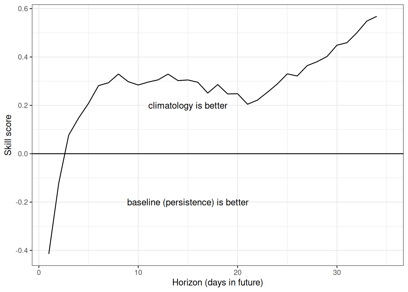

11.7 Take homes

Different metrics evaluate different components of the forecast. Be sure to match your evaluation metric to the aspects of the forecast that meet the forecast user’s needs.

11.8 Reading

Simonis, J. L., White, E. P., & Ernest, S. K. M. (2021). Evaluating probabilistic ecological forecasts. Ecology, 102(8). https://doi.org/10.1002/ecy.3431

11.9 Problem Set

If you have forecast submissions the scores from your submitted forecasts and the climatology and persistence forecasts. If you have not submitted forecasts, select a model from the catalog to answer the questions

Create a new Quarto document to answer the questions below, using a mix of code and text.

11.10 Part 1: a single forecast

1. Access climatology, persistence, and a model of your choice from the NEON forecast STAC catalog for a specific reference_datetime where all three models are available (https://radiantearth.github.io/stac-browser/#/external/raw.githubusercontent.com/eco4cast/neon4cast-catalog/main/forecasts/collection.json). If you have been iteratively submitting your own model, you are welcome to use that model.

You may need to replace the example code in the STAC catalog with the following to avoid errors:

all_results <- duckdbfs::open_dataset("s3://bio230014-bucket01/challenges/forecasts/bundled-parquet/project_id=neon4cast/duration=P1D/variable=temperature", s3_endpoint="sdsc.osn.xsede.org", anonymous=TRUE)

2. Access the observations that are associated with your selected target variable (see https://www.neon4cast.org).
3. Plot the three forecasts using a ribbon plot on the same graph. Add the observations. The x-axis should be datetime and the y-axis the forecasted value.
4. Based on visual inspection of your plot for the one forecast period, how does each model differ in capacity to represent the observations?
5. Based on visual inspection of your plot, how does the uncertainty of each model forecast differ in its capacity to capture the observations?
6. Using the scoringRules package, calculate the CRPS for each model and forecasted datetime.
7. Plot how CRPS vs. datetime for each model on the same plot and compare the results to your visual inspections in questions 4 and 5.

11.11 Part 2: multiple forecasts

8. Download all the forecasts generated by climatology, persistence, and your chosen model (your will have multiple reference_datetimes).
   
9. Calculate the mean CRPS for climatology, persistence, and your model for all reference datetimes and horizons. Which model has the lower score when you consider all submissions?
10. Do you think you have enough information from the mean CRPS score to determine the “best” model? If not, what is needed to better characterize the best-performing model?

Commit your QMD and render HTML to your GitHub repository that you used in Chapter 10.

Gneiting, Tilmann, and Adrian E Raftery. 2007. “Strictly Proper Scoring Rules, Prediction, and Estimation.” Journal of the American Statistical Association 102 (477): 359–78. https://doi.org/10.1198/016214506000001437.