if(file.exists("data/PF_analysis_1.Rdata")){
  load("data/PF_analysis_1.Rdata")
}else{
  load("data/PF_analysis_0.Rdata")
}
ens_members <- dim(analysis$forecast)[2]21 Forecast - analysis cycle
21.1 Step 1: Set initial conditions and parameter distributions
We will start our forecast-analysis cycle by running the model with a particle filter over some time in the past. This is designed to spin up the model and set the initial states and parameters for a forecast.
Now we are going to generate a forecast that starts from our last saved forecast. First, load the forecast into memory so we can access its initial conditions and parameters.
21.2 Step 2: Get latest data
The latest observation data is available by running Chapter 18 and reading in the CSV. You will need to re-run the code in Chapter 18 if you want to update the observations outside the automatic build of this book.
obs <- read_csv("data/site_carbon_data.csv", show_col_types = FALSE)21.3 Step 3: Generate forecast
This example introduces the concept of a “look back”. This is stepping back in time to restart the particle filter so it can assimilate any data made available since the last time the particle filter was run. The “look back” is important because many observations have delays before becoming available (latency). NEON flux data can have a latency of 5 days to 1.5 months. MODIS LAI is an 8-day average, so it has an 8-day latency.
Here, we use a 30-day “look back”. Since our forecast horizon is 30 days, the total number of simulation days is 30 + 30. Our reference_datetime is today.
site <- "OSBS"
look_back <- 30
horizon <- 30
reference_datetime <- Sys.Date()
#reference_datetime <- as_date("2025-12-15")
sim_dates <- seq(reference_datetime - look_back, length.out = look_back + horizon, by = "1 day")
Since yesterday’s forecast also included a 30-day “look back”, we can find the first day of our simulation (30 days ago) in the last saved analysis and use it as initial conditions.
index <- which(analysis$sim_dates == sim_dates[1])The use of the look-back requires combining the “historical” weather and future weather into a single input data frame.
inputs_past <- get_historical_met(site = site, sim_dates[1:(look_back-2)], use_mean = FALSE)
inputs_future <- get_forecast_met(site = site, sim_dates[(look_back-1):length(sim_dates)], use_mean = FALSE)
inputs <- bind_rows(inputs_past, inputs_future)
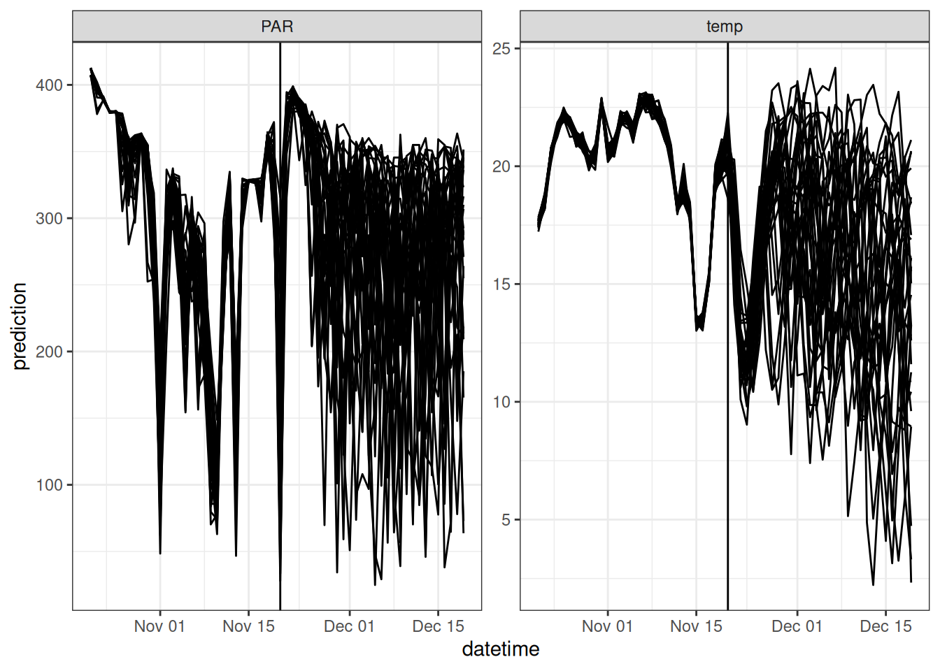
inputs_ensemble <- assign_met_ensembles(inputs, ens_members)The combined weather drivers, along with the concept of the “look back”, are shown in the figure below. The vertical line marks the transition from the “look back” period to the future.
The object with yesterday’s forecast also has the parameter values. Load the fixed parameter values and initialize the parameters that are being fit by the particle filter with the values from the analysis.
params <- analysis$params

num_pars <- 2
fit_params <- array(NA, dim = c(length(sim_dates) ,ens_members , num_pars))
fit_params[1, , 1] <- analysis$fit_params[index, ,1]
fit_params[1, , 2] <- analysis$fit_params[index, ,2]
Initialize the states using the states from the analysis that occurred on the index simulation date in the previous run through the particle filter.
#Set initial conditions
forecast <- array(NA, dim = c(length(sim_dates), ens_members, 12)) #12 is the number of outputs
forecast[1, , 1] <- analysis$forecast[index, ,1]
forecast[1, , 2] <- analysis$forecast[index, ,2]
forecast[1, , 3] <- analysis$forecast[index, ,3]

wt <- array(1, dim = c(length(sim_dates), ens_members))
wt[1, ] <- analysis$wt[index, ]
Run the particle filter (over the “look back” days) that transitions to a forecast (which is the same as the particle filter without data)
for(t in 2:length(sim_dates)){

  fit_params[t, , 1] <- rnorm(ens_members, fit_params[t-1, ,1], sd = 0.0005)
  fit_params[t, , 2] <- rnorm(ens_members, fit_params[t-1, ,2], sd = 0.00005)

  params$alpha  <- fit_params[t, , 1]
  params$Rbasal  <- fit_params[t, , 2]

  if(t > 1){

  forecast[t, , ]  <- forest_model(t,
                                   states = matrix(forecast[t-1 , , 1:3], nrow = ens_members) ,
                                   parms = params,
                                   inputs = matrix(inputs_ensemble[t , , ], nrow = ens_members))
  }

  analysis <- particle_filter(t, forecast, obs, sim_dates, wt, fit_params,
                              variables = c("lai", "wood", "som", "nee"),
                              sds = c(0.1, 1, 20, 0.005))

  forecast <- analysis$forecast
  fit_params <- analysis$fit_params
  wt <- analysis$wt
}
21.4 Step 4: Save forecast and data assimilation output
Convert forecast to a dataframe.
output_df <- output_to_df(forecast, sim_dates, sim_name = "simple_forest_model")forecast_weighted <- array(NA, dim = c(length(sim_dates), ens_members, 12))
params_weighted <- array(NA, dim = c(length(sim_dates) ,ens_members , num_pars))
for(t in 1:length(sim_dates)){
wt_norm <- wt[t, ]/sum(wt[t, ])
resample_index <- sample(1:ens_members, ens_members, replace = TRUE, prob = wt_norm )
forecast_weighted[t, , ] <- forecast[t, resample_index, 1:12]
params_weighted[t, , ] <- fit_params[t,resample_index, ]
}
output_df <- output_to_df(forecast_weighted, sim_dates, sim_name = "simple_forest_model")
parameter_df <- parameters_to_df(params_weighted, sim_dates, sim_name = "simple_forest_model", param_names = c("alpha","Rbasal"))Figure 21.1 is a visualization of the forecast. The vertical line marks the transition from the look-back period to the future.
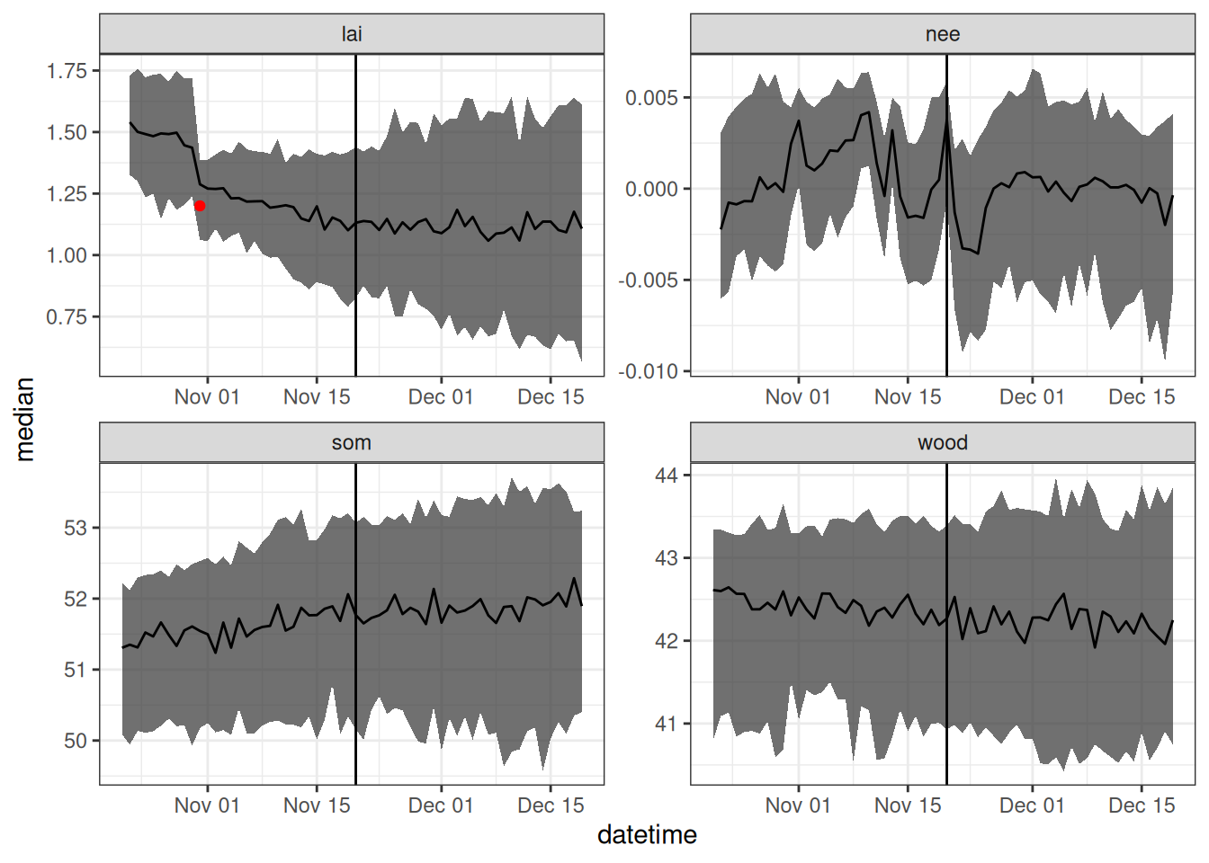
Save the states and weights for use as initial conditions in the next forecast.
analysis$params <- params
save(analysis, file = "data/PF_analysis_1.Rdata")
Convert to the format and units required by the NEON Ecological Forecasting Challenge
efi_output <- output_df |>
  mutate(datetime = as_datetime(datetime),
         model_id = "bookcast_forest",
         duration = "P1D",
         project_id = "neon4cast",
         site_id = site,
         family = "ensemble",
         reference_datetime = as_datetime(reference_datetime)) |>
  rename(parameter = ensemble) |>
  filter(datetime >= reference_datetime) |>
  filter(variable == "nee") |>
  mutate(prediction = prediction  / 0.01) #Convert from MgC/ha/Day to gC/m2/day
Write the forecast to a CSV file
file_name <- paste0("data/terrestrial_daily-", reference_datetime, "-bookcast_forest.csv")
write_csv(efi_output, file_name)
and submit to the Challenge. The submission uses the submit function in the neon4cast package(remotes::install_github("eco4cast/neon4cast"))
neon4cast::submit(file_name, ask = FALSE)validating that file matches required standarddata/terrestrial_daily-2026-06-07-bookcast_forest.csv✔ file has model_id column
✔ only one unique value in the model_id column
✔ forecasted variables found correct variable + prediction column
✔ nee is a valid variable name
✔ file has correct family and parameter columns
✔ only one unique value in the family column
✔ file has site_id column
✔ file has datetime column
✔ file has correct datetime column
✔ file has correct duration column
✔ file has project_id column
✔ file has reference_datetime column
Forecast format is valid
Thank you for submitting!21.5 Step 5: Repeat Steps 2 - 4
Wait a day, then use yesterday’s analysis today as initial conditions and parameter distributions. This particular forecast uses GitHub Actions to automatically render the book each day; rendering this chapter generates, saves, and submits the latest forecast.
load("data/PF_analysis_1.Rdata")21.6 Additional example
I recommend looking at a tutorial created by Mike Dietze that has many of the particle filter concepts used here. It is a similar process model that runs at the 30-minute time step. The tutorial is more advanced in its use of parameter priors and shows how to forecast across multiple sites.